Table Of Content
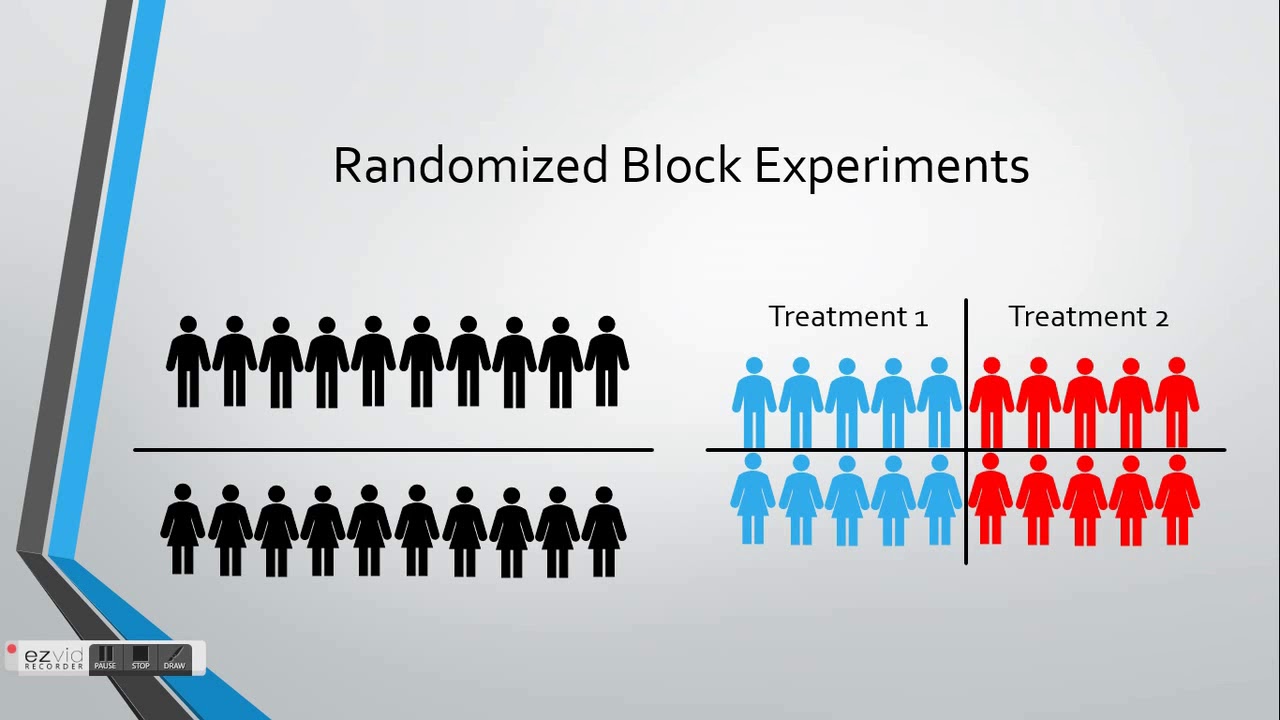
One possible alternative is to treat it like a factorial ANOVA where the independent variables are allowed to interact with each other. In randomized block design, the control technique is done through the design itself. First the researchers need to identify a potential control variable that most likely has an effect on the dependent variable. Researchers will group participants who are similar on this control variable together into blocks. This control variable is called a blocking variable in the randomized block design. The purpose of the randomized block design is to form groups that are homogeneous on the blocking variable, and thus can be compared with each other based on the independent variable.
Magnitude of Effects
For example, consider if the drug was a diet pill and the researchers wanted to test the effect of the diet pills on weight loss. The explanatory variable is the diet pill and the response variable is the amount of weight loss. Although the sex of the patient is not the main focus of the experiment—the effect of the drug is—it is possible that the sex of the individual will affect the amount of weight lost. This ANOVA table provides all the information that we need to (1) test hypotheses and (2) assess the magnitude of treatment effects. However, a nuisance variable that will likely cause variation is gender.
ANOVA Summary Table
To address nuisance variables, researchers can employ different methods such as blocking or randomization. Blocking involves grouping experimental units based on levels of the nuisance variable to control for its influence. Randomization helps distribute the effects of nuisance variables evenly across treatment groups. A special case is the so-calledLatin Square design where we have two blockfactors and one treatment factor having \(g\) levels each (yes, all of them!).Hence, this is a very restrictive assumption.
Mathematical Model
The simplest case is where you only have 2 treatments and you want to give each subject both treatments. Here as with all crossover designs we have to worry about carryover effects. As the treatments were assigned you should have noticed that the treatments have become confounded with the days. Days of the week are not all the same, Monday is not always the best day of the week! Just like any other factor not included in the design you hope it is not important or you would have included it into the experiment in the first place. In this factory you have four machines and four operators to conduct your experiment.

Select appropriate blocking factors
Even though we are not interested in the blocking variable, we know based on the theoretical and/or empirical evidence that the blocking variable has an impact on the dependent variable. By adding it into the model, we reduce its likelihood to confound the effect of the treatment (independent variable) on the dependent variable. If the blocking variable (or the groupings of the block) has little effect on the dependent variable, the results will be biased and inaccurate. We are less likely to detect an effect of the treatment on the outcome variable if there is one. Comparing the two ANOVA tables, we see that the MSE in RCBD has decreased considerably in comparison to the CRD. This reduction in MSE can be viewed as the partition in SSE for the CRD (61.033) into SSBlock + SSE (53.32 + 7.715, respectively).
Understanding and visualizing ResNets by Pablo Ruiz - Towards Data Science
Understanding and visualizing ResNets by Pablo Ruiz.
Posted: Thu, 18 Oct 2018 13:37:21 GMT [source]
To answer these questions, the researcher uses analysis of variance. In that sense, Latin Square designs are useful building blocksof more complex designs, see for example Kuehl (2000). That is , if the experiment was repeated, a new sample of i batches would be selected,d yielding new values for \(\rho_1, \rho_2,...,\rho_i\) then. Here is Dr. Shumway stepping through this experimental design in the greenhouse.
Table
When we can utilize these ideal designs, which have nice simple structure, the analysis is still very simple, and the designs are quite efficient in terms of power and reducing the error variation. The single design we looked at so far is the completely randomized design (CRD) where we only have a single factor. In the CRD setting we simply randomly assign the treatments to the available experimental units in our experiment. We have four different varieties of rice; varieties A, B, C, and D. So, imagine each of these blocks as a rice field or patty on a farm somewhere.
Ok, with this scenario in mind, let's consider three cases that are relevant and each case requires a different model to analyze. The cases are determined by whether or not the blocking factors are the same or different across the replicated squares. The treatments are going to be the same but the question is whether the levels of the blocking factors remain the same. Whenever, you have more than one blocking factor a Latin square design will allow you to remove the variation for these two sources from the error variation. So, consider we had a plot of land, we might have blocked it in columns and rows, i.e. each row is a level of the row factor, and each column is a level of the column factor. We can remove the variation from our measured response in both directions if we consider both rows and columns as factors in our design.
Here we have two pairs occurring together 2 times and the other four pairs occurring together 0 times. Therefore, this is not a balanced incomplete block design (BIBD). Here is a plot of the least square means for treatment and period. We can see in the table below that the other blocking factor, cow, is also highly significant. Crossover designs use the same experimental unit for multiple treatments.
Variability between blocks can be large, since we will remove this source of variability, whereas variability within a block should be relatively small. In general, a block is a specific level of the nuisance factor. Back to the hardness testing example, the experimenter may very well want to test the tips across specimens of various hardness levels. To conduct this experiment as a RCBD, we assign all 4 tips to each specimen.
For example, suppose each individual has a certain amount of innate discipline that they can draw upon to lose more weight. Since discipline is hard to measure, it’s not included as a blocking factor in the study but one way to control for it is to use randomization. In the previous example, gender was a known nuisance variable that researchers knew affected weight loss. By placing the individuals into blocks, the relationship between the new diet and weight loss became more clear since we were able to control for the nuisance variable of gender. Unfortunately nuisance variables often arise in experimental studies, which are variables that effect the relationship between the explanatory and response variable but are of no interest to researchers.
In the most basic form, we assume that we do not have replicateswithin a block. This means that we only observe every treatment once in eachblock. A farmer possesses five plots of land where he wishes to cultivate corn. He wants to run an experiment since he has two kinds of corn and two types of fertilizer. Moreover, he knows that his plots are quite heterogeneous regarding sunshine, and therefore a systematic error could arise if sunshine does indeed facilitate corn cultivation.
For most of our examples, GLM will be a useful tool for analyzing and getting the analysis of variance summary table. Even if you are unsure whether your data are orthogonal, one way to check if you simply made a mistake in entering your data is by checking whether the sequential sums of squares agree with the adjusted sums of squares. If this point is missing we can substitute x, calculate the sum of squares residuals, and solve for x which minimizes the error and gives us a point based on all the other data and the two-way model. We sometimes call this an imputed point, where you use the least squares approach to estimate this missing data point. To conduct this experiment as a RCBD, we need to assign all 4 pressures at random to each of the 6 batches of resin.


No comments:
Post a Comment